River network analysis use case
Welcome to the "Railway use case" page. Here is information on how you can use the plugin to analyze the railways network and prepare visualizations.
Important tip!
Before starting to use the algorithm, please make sure that the project uses metric projection. Also the layers used in the calculation (both linear and point layers) should be converted to this projection.
Experiment setup
- QGIS Desktop 3.34.3
- Windows
- Date: 07.02.2024
- Data: Finland railways vector layer - see fin_rails in the repository
Load vector data and assign projection WGS 84 / UTM zone 35N for the project:
- Project:
Project-Properties-CRS-WGS 84 / UTM zone 35N;
There is no need to reproject layer because it is already has CRS WGS 84 / UTM zone 35N.
turn on Open Street Map: Web - QuickWebServices - OSM - OSM Standard. And obtain the following initial picture:
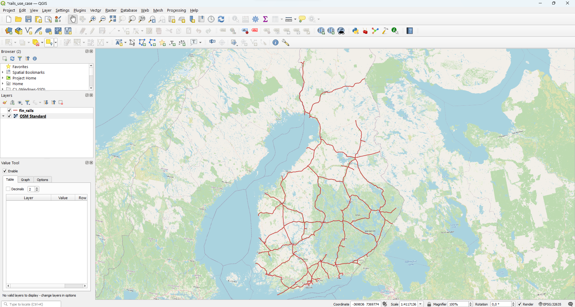
In front of you is the railroad network of Finland. Let's try to look at this network as a "river network". Indeed, there are many similarities: Finland's largest city, Helsinki, is located in the south of the country. The rail network converges to the capital in one way or another, as Helsinki is crucial logistics hub.
Thus, choose start point (Helsinki) and launch the algorithm - Shreve value are shown via line size:
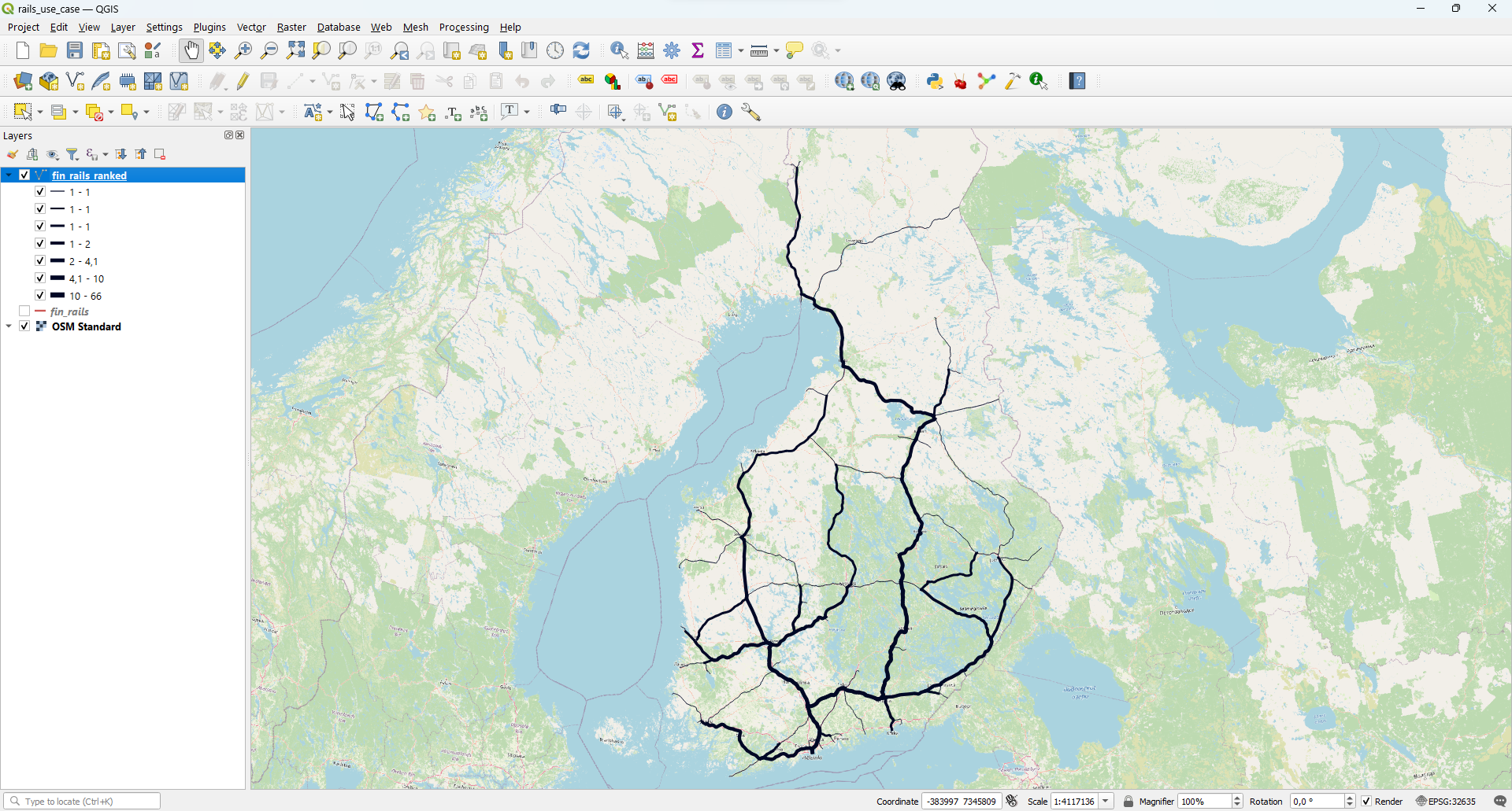
The algorithm will assign four parameters to each river segment: ValueShreve, ValueStrahler, Rank, Distance
After that, visualizations can be prepared via fin_rails_ranked - Properties - Symbology - Graduated.
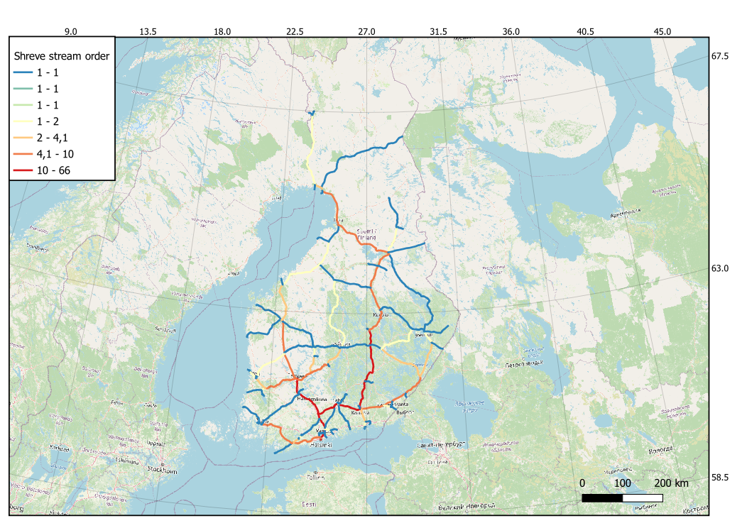
Shreve stream order
Visualize "ValueShreve" column and prepare a map
Strahler stream order
Visualize "ValueStrahler" column and prepare a map

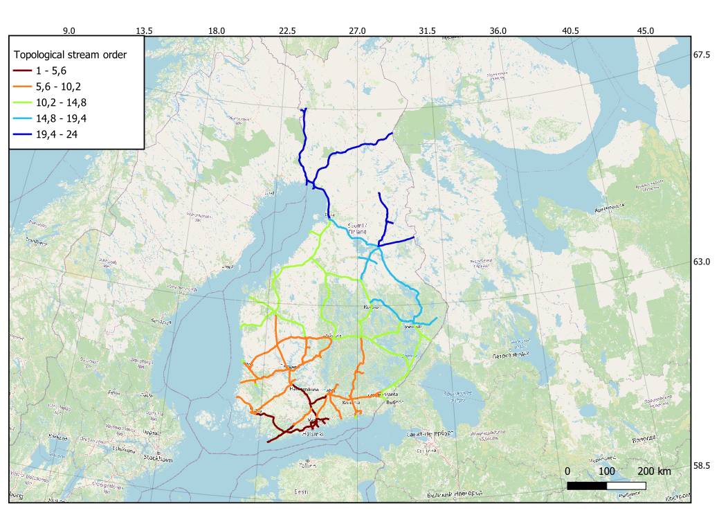
Topological stream order
Visualize "Rank" column and prepare a map